Microsoft Excel is great for working with numerical data. Let’s get started with some some basic starter tips to get you going!
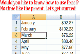
Let’s take an example of tracking a utility bill that you may have over the course of a year. So in the first column we will want the months displayed. In the second column, let’s put the amount paid. At the bottom of the list, we’ll add up the column to get a total.
I’m all about shortcuts. You are going to learn a few shortcuts from me right now!
Let’s start with the A column. You could type in each of the names of the 12 months, but don’t. You only need to type January in the A1 cell and then let Excel fill in the rest. After you type in the January text, make sure that the cell is highlighted and then notice the lower-right corner of the cell. Do you see the little square there? (it is technically called a “handle“) Take your mouse and drag from that handle downward to fill in a total of 12 cells. Done! Your months are filled in. Auto-fill senses what is in the cells and if it sees a pattern, it will complete it for you.

The A column may feel a little cramped and we should widen it out some to make it better sized based on the content that is now in it. To do that, grab the bar at the column header area and drag it over some to pick a better width.

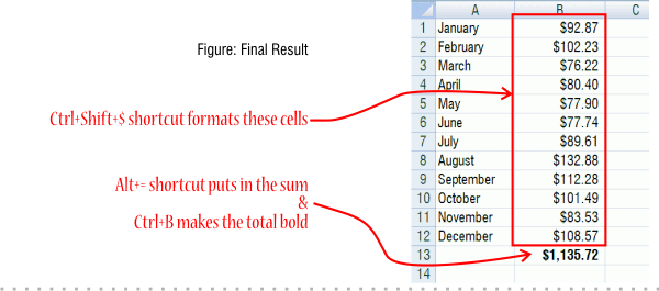
Now let’s take the B column as the amount paid. Start typing your first amount in B1. You can press Enter or use your down arrow to type in the different amounts in the subsequent cells. The basic formatting will be ok, but it will be much better if it is in currency format. So in instead of a number reading like 77.9 it will show as $77.90. So the next shortcut is to highlight all the cells to use this format and then use the Ctrl+Shift+$ key combo to format as currency (that is: hold down Ctrl+Shift together first, then press the $ key)
Next, let’s do our total. Select the B13 cell and press the Alt+= keyboard shortcut (that is while holding down the Alt key, press =). Excel knows you want the sum formula and it also auto-detects the range to sum as all the cells connected directly above. Press Enter and you’ve got it. Maybe then select the cell one more time and press Ctrl+B to make it bold (sorry Mac users for using windows key references, you probably have something like the Command key to do the same thing).

Were you able to follow along. Congratulations, you just did some of the basic spreadsheet types of tasks like auto-fill and formatting cells and getting a total. Stay tuned to this blog for more Excel tips!


